Bertrand paradox (probability)

For other paradoxes by Joseph Bertrand, see Bertrand's paradox (disambiguation).

The Bertrand paradox is a problem within the classical interpretation of probability theory. Joseph Bertrand introduced it in his work Calcul des probabilités (1889) as an example to show that the principle of indifference may not produce definite, well-defined results for probabilities if it is applied uncritically when the domain of possibilities is infinite.

Bertrand's formulation of the problem

The Bertrand paradox is generally presented as follows: Consider an equilateral triangle that is inscribed in a circle. Suppose a chord of the circle is chosen at random. What is the probability that the chord is longer than a side of the triangle?

Bertrand gave three arguments (each using the principle of indifference), all apparently valid yet yielding different results:

1. 

   Random chords, selection method 1; red = longer than triangle side, blue = shorter

   The "random endpoints" method: Choose two random points on the circumference of the circle and draw the chord joining them. To calculate the probability in question imagine the triangle rotated so its vertex coincides with one of the chord endpoints. Observe that if the other chord endpoint lies on the arc between the endpoints of the triangle side opposite the first point, the chord is longer than a side of the triangle. The length of the arc is one third of the circumference of the circle, therefore the probability that a random chord is longer than a side of the inscribed triangle is ⁠1/3⁠.


Calculation example 1

The unit circle $S_{1}={\big \{}u\in \mathrm {\mathbb {R} } ^{2}/\|u\|=1$, $\|.\|$ the Euclidean norm ${\big \}}$ is homeomorphic to $\mathrm {\mathbb {R} /\mathbb {Z} }$. On $\mathrm {\mathbb {R} /\mathbb {Z} }$ we use the measure $\delta$ of density 1, which corresponds to the length of an arc divided by $2\pi$ modulo 1, on $\mathrm {\mathbb {R} /\mathbb {Z} }$. So $\delta {\big (}\mathrm {\mathbb {R} /\mathbb {Z} } {\big )}=\int _{\mathrm {\mathbb {R} /\mathbb {Z} } }d\delta =1$ . (See hereunder in “a way out” Miscellaneous chapter for a formal definition).

We consider the unit disk $D_{1}$ of center $(1,$ $0)$ in the affine Euclidean plane with the canonical basis and for it, we define a chord as the intersection ${\mathcal {D}}_{1}\cap D_{\alpha }$ where $D_{\alpha }$ is a straight line whose equation in the plane is $y=\tan(\alpha )x$ if $\alpha \in {\Big [}0\mathrm {,} {\phantom {a}}{\frac {\pi }{2}}{\Big [}=I_{1}$, and $D_{\frac {\pi }{2}}{\underset {\mathrm {def.} }{=}}{\big \{}(x\mathrm {,} {\phantom {a}}y)\in \mathbb {R} ^{2},x=0{\big \}}$.



So basically a chord is an element of $\Omega ={\overline {I_{1}}}$x$\mathrm {\mathbb {R} /\mathbb {Z} }$, let $T$ be the probability space $(\Omega \mathrm {,} {\phantom {a}}{\mathcal {P}}(\Omega )\mathrm {,} {\phantom {a}}P)$ where we choose $P$ as the product probability of constant density hence of density ${\frac {2}{\pi }}1_{\Omega }$, (If $x\in \Omega$ then $1_{\Omega }(x)=1$ and $=0$ otherwise) which using Fubbini since the measure $P$ is finite, yields:


$P{\Big (}{\Big [}0\mathrm {,} {\phantom {a}}{\frac {\pi }{6}}{\Big ]}$x$\mathrm {\mathbb {R} /\mathbb {Z} } {\Big )}=$
$\int _{{\Big [}0\mathrm {,} {\phantom {a}}{\frac {\pi }{6}}{\Big ]}\mathrm {x} \mathrm {\mathbb {R} /\mathbb {Z} } }dP={\frac {2}{\pi }}\int _{{\Big [}0\mathrm {,} {\phantom {a}}{\frac {\pi }{6}}{\Big ]}}d\alpha \int _{\mathrm {\mathbb {R} /\mathbb {Z} } }d\delta ={\frac {1}{3}}$




2. 

   Random chords, selection method 2

   The "random radial point" method: Choose a radius of the circle, choose a point on the radius and construct the chord through this point and perpendicular to the radius. To calculate the probability in question imagine the triangle rotated so a side is perpendicular to the radius. The chord is longer than a side of the triangle if the chosen point is nearer the center of the circle than the point where the side of the triangle intersects the radius. The side of the triangle bisects the radius, therefore the probability a random chord is longer than a side of the inscribed triangle is ⁠1/2⁠.


Calculation example 2

The unit circle $S_{1}={\big \{}u\in \mathrm {\mathbb {R} } ^{2}/\|u\|=1$, $\|.\|$ the Euclidean norm ${\big \}}$ is homeomorphic to $\mathrm {\mathbb {R} /\mathbb {Z} }$. On $\mathrm {\mathbb {R} /\mathbb {Z} }$ we use the measure $\delta$ of density 1, which corresponds to the length divided by $2\pi$ of an arc modulo 1, on $\mathrm {\mathbb {R} /\mathbb {Z} }$. So $\delta {\big (}\mathrm {\mathbb {R} /\mathbb {Z} } {\big )}=\int _{\mathrm {\mathbb {R} /\mathbb {Z} } }d\delta =1$. (See hereunder in “a way out” Miscellaneous chapter for a formal definition)

We consider the unit disk $D_{1}$ of center $O=(0\mathrm {,} {\phantom {a}}0)$ in the affine Euclidean plane with the canonical basis. And for $r\in [0\mathrm {,} {\phantom {a}}1]=I$ we define a chord as the intersection ${\mathcal {D}}_{1}\cap D_{r}$ where $D_{r}$ is a straight line whose equation in the plane is ${\overrightarrow {\omega M}}.{\vec {u}}=0$ with ${\vec {u}}=(\cos(2\pi \theta )\mathrm {,} {\phantom {a}}\sin(2\pi \theta ))\in S_{1}\thicksim \mathbb {R} /\mathbb {Z}$, $\omega =O+r{\vec {u}}$

So basically a chord is an element of $\Omega =I$x$\mathrm {\mathbb {R} /\mathbb {Z} }$, let $T$ be the probability space $(\Omega \mathrm {,} {\phantom {a}}{\mathcal {P}}(\Omega )\mathrm {,} {\phantom {a}}P)$ where we choose $P$ as the product probability of constant density hence of density $1_{\Omega }$, (If $x\in \Omega$ then $1_{\Omega }(x)=1$ and $=0$ otherwise) which using Fubbini since the measure $P$ is finite, yields:

$P{\Big (}{\Big [}0$, ${\frac {1}{2}}{\Big ]}$x$\mathrm {\mathbb {R} /\mathbb {Z} } {\Big )}=$
$\int _{{\Big [}0\mathrm {,} {\frac {1}{2}}{\Big ]}\mathrm {x} \mathrm {\mathbb {R} /\mathbb {Z} } }dP=\int _{{\Big [}0\mathrm {,} {\frac {1}{2}}{\Big ]}}dr\int _{\mathrm {\mathbb {R} /\mathbb {Z} } }d\delta ={\frac {1}{2}}$




3. 

   Random chords, selection method 3

   The "random midpoint" method: Choose a point anywhere within the circle and construct a chord with the chosen point as its midpoint. The chord is longer than a side of the inscribed triangle if the chosen point falls within a concentric circle of radius ⁠1/2⁠ the radius of the larger circle. The area of the smaller circle is one fourth the area of the larger circle, therefore the probability a random chord is longer than a side of the inscribed triangle is ⁠1/4⁠.


Calculation example 3

A chord is defined as a point in a unit disk, and the event we look for is ${\mathcal {D}}_{\frac {1}{2}}={\big \{}\|u\|\leq {\frac {1}{2}}$ $/$ $u\in \mathrm {\mathbb {R} } ^{2}\mathrm {,} {\phantom {a}}\|.\|$ the Euclidean norm ${\big \}}$ considering the probability space $({\mathcal {D}}_{1}\mathrm {,} {\phantom {a}}{\mathcal {P}}({\mathcal {D}}_{1})\mathrm {,} {\phantom {a}}P)$ where we choose $P$ as the probability of constant density hence of density ${\frac {1}{\pi }}1_{{\mathcal {D}}_{1}}$ (If $x\in {\mathcal {D}}_{1}$ then $1_{{\mathcal {D}}_{1}}(x)=1$ and $=0$ otherwise) renders:

$P{\Big (}{\mathcal {D}}_{\frac {1}{2}}{\Big )}=\int _{{\mathcal {D}}_{\frac {1}{2}}}{\frac {1}{\pi }}dxdy={\Big (}{\frac {1}{2}}{\Big )}^{2}$

These three selection methods differ as to the weight they give to chords which are diameters. This issue can be avoided by "regularizing" the problem so as to exclude diameters, without affecting the resulting probabilities. But as presented above, in method 1, each chord can be chosen in exactly one way, regardless of whether or not it is a diameter; in method 2, each diameter can be chosen in two ways, whereas each other chord can be chosen in only one way; and in method 3, each choice of midpoint corresponds to a single chord, except the center of the circle, which is the midpoint of all the diameters.

Scatterplots showing simulated Bertrand distributions,
midpoints/chords chosen at random using the above methods.

Midpoints of the chords chosen at random using method 1	Midpoints of the chords chosen at random using method 2	Midpoints of the chords chosen at random using method 3
Chords chosen at random, method 1	Chords chosen at random, method 2	Chords chosen at random, method 3

Other selection methods have been found. In fact, there exists an infinite family of them.
See more examples below:

4. A chord defined as an angle and a length

The unit circle $S_{1}={\big \{}u\in \mathrm {\mathbb {R} } ^{2}/\|u\|=1$, $\|.\|$ the Euclidean norm ${\big \}}$ is homeomorphic to $\mathrm {\mathbb {R} /\mathbb {Z} }$. On $\mathrm {\mathbb {R} /\mathbb {Z} }$ we use the measure $\delta$ of density 1, which corresponds to the length divided by $2\pi$ of an arc modulo 1, on $\mathrm {\mathbb {R} /\mathbb {Z} }$. So $\delta {\big (}\mathrm {\mathbb {R} /\mathbb {Z} } {\big )}=\int _{\mathrm {\mathbb {R} /\mathbb {Z} } }d\delta =1$. (See hereunder in “a way out” Miscellaneous chapter for a formal definition)

We define a chord (of length smaller than 2) in a unit disk as a couple (length, orientation) in $\Omega =[0\mathrm {,} {\phantom {a}}2[\mathrm {x} S_{1}=[0\mathrm {,} {\phantom {a}}2[\mathrm {x} \mathrm {\mathbb {R} /\mathbb {Z} }$

A chord defined as an angle and a length

So basically a chord is an element of $\Omega =[0\mathrm {,} {\phantom {a}}2[$x$\mathrm {\mathbb {R} /\mathbb {Z} }$, let $T$ be the probability space $(\Omega \mathrm {,} {\phantom {a}}{\mathcal {P}}(\Omega )\mathrm {,} {\phantom {a}}P)$ where we choose $P$ as the product probability of constant density hence of density ${\frac {1}{2}}1_{\Omega }$, (If $x\in \Omega$ then $1_{\Omega }(x)=1$ and $=0$ otherwise) which using Fubbini since the measure $P$ is finite, yields:

$P{\Big (}{\big [}{\sqrt {3}}\mathrm {,} 2{\big [}\mathrm {x} \mathrm {\mathbb {R} /\mathbb {Z} } {\Big )}=\int _{{{\big [}{\sqrt {3}}\mathrm {,} 2{\big [}}\mathrm {x} \mathrm {\mathbb {R} /\mathbb {Z} } }dP={\frac {1}{2}}\int _{{\big [}{\sqrt {3}}\mathrm {,} 2{\big [}}dx\int _{\mathrm {\mathbb {R} /\mathbb {Z} } }d\delta =1-{\frac {\sqrt {3}}{2}}$

Since the measure of diameters in the disk are of null measure for the Borel-Lebesgue measure we can consider $\Omega =[0\mathrm {,} {\phantom {a}}2]\mathrm {x} S_{1}$ instead with exactly the same result.

5. A chord defined as a gradient

Let’s choose a probability $q\in ]0\mathrm {,} {\phantom {a}}{\frac {1}{2}}[$. The unit circle $S_{1}={\big \{}u\in \mathrm {\mathbb {R} } ^{2}/\|u\|=1$, $\|.\|$ the Euclidean norm ${\big \}}$ is homeomorphic to $\mathrm {\mathbb {R} /\mathbb {Z} }$. On $\mathrm {\mathbb {R} /\mathbb {Z} }$ we use the measure $\delta$ of density 1, which corresponds to the length divided by $2\pi$ of an arc modulo 1, on $\mathrm {\mathbb {R} /\mathbb {Z} }$. So $\delta {\big (}\mathrm {\mathbb {R} /\mathbb {Z} } {\big )}=\int _{\mathrm {\mathbb {R} /\mathbb {Z} } }d\delta =1$. (See hereunder in “a way out” Miscellaneous chapter for a formal definition)

Let’s consider a unit disk ${\mathcal {D}}_{k}$ of center $K=(k\mathrm {,} {\phantom {a}}0)\mathrm {,} {\phantom {a}}k\in ]1\mathrm {,} {\phantom {a}}+\infty [$ in the Euclidean plane with the canonical basis, and a straight line $D_{\alpha }$ whose equation is $y=\alpha x$ where $\alpha \in {\bigg [}0\mathrm {,} {\phantom {a}}{\frac {1}{(k^{2}-1)^{2}}}{\bigg ]}=I_{k}$, then we define a chord as the intersection ${\mathcal {D}}_{k}\cap D_{\alpha }$ for a given $\alpha \in I_{k}$, so basically in the Bertrand’s experiment a chord is an element of $\Omega _{k}=I_{k}$x$\mathrm {\mathbb {R} /\mathbb {Z} }$, let $T$ be the probability space $(\Omega _{k}\mathrm {,} {\phantom {a}}{\mathcal {P}}(\Omega _{k})\mathrm {,} {\phantom {a}}P)$ where we choose $P$ as the product probability of constant density hence of density ${\frac {1}{\mu (I_{k})}}1_{\Omega _{k}}$ (If $x\in \Omega _{k}$ then $1_{\Omega _{k}(x)}=1$ and $=0$ otherwise) where $\mu$ is the Borel-Lebesgue measure.

A chord defined as a gradient

Let $[M_{1}\mathrm {,} {\phantom {a}}M_{2}]$ be a chord of ${\mathcal {D}}_{k}\cap D_{\alpha }$, We consider the function $f_{k}$ which maps $\alpha \in I_{k}$ to $f_{k}(\alpha )=M_{1}M_{2}{\underset {\mathrm {def.} }{=}}\mathrm {d} (M_{1},M_{2})$ (d the Euclidean distance), $f_{k}$ is continuous and strictly decreasing on $I_{k}$,

Calculation of $f_{k}$ 

$M_{j}=K+\mathrm {exp} (i\theta _{j})=(x_{j}\mathrm {,} {\phantom {a}}\alpha x_{j})$ for $j=1$ or $2$ with $i^{2}=-1\mathrm {,} {\phantom {a}}\mathrm {\mathbb {R} } ^{2}\thicksim \mathrm {\mathbb {C} }$. $x_{j}$ are the roots of the polynomial: $(\alpha X)^{2}+(X-k)^{2}-1=(1+\alpha ^{2})X^{2}-2kX+k^{2}-1$ whose half discriminant is: $\Delta ={\Big (}k^{2}+(1-k^{2})(1+\alpha ^{2}){\Big )}^{\frac {1}{2}}={\Big (}1+(1-k^{2})\alpha ^{2}{\Big )}^{\frac {1}{2}}$ We posit $\tan ^{-1}(\alpha )=\theta {\big (}$ Thus $\cos(\theta )={\frac {1}{(1+\alpha ^{2})^{\frac {1}{2}}}}{\big )}$, we have: ${\frac {\sin(\theta _{j})}{OM_{j}}}={\frac {\sin(\theta )}{1}}$ henceforth $M_{1}M_{2}=\left|OM_{1}-OM_{2}\right|={\frac {1}{\left|\sin(\theta )\right|}}\left|y_{2}-y_{1}\right|={\frac {\alpha }{\sin(\theta )}}\left|x_{2}-x_{1}\right|=(1+\alpha ^{2})^{\frac {1}{2}}2{\frac {\Delta }{1+\alpha ^{2}}}$, result valid even for $\theta =0$ which leads to: $f_{k}(\alpha )={\frac {2{\Big (}1+(1-k^{2})\alpha ^{2}{\Big )}^{\frac {1}{2}}}{(1+\alpha ^{2})^{\frac {1}{2}}}}$

End of calculation of $f_{k}$ 

And the probability we look for is: $Q=P{\Big (}{\big [}0\mathrm {,} f_{k}^{-1}({\sqrt {3}}){\big ]}\mathrm {x} \mathrm {\mathbb {R} /\mathbb {Z} } {\Big )}=\int _{{{\big [}0\mathrm {,} f_{k}^{-1}({\sqrt {3}}){\big ]}}\mathrm {x} \mathrm {\mathbb {R} /\mathbb {Z} } }dP=g(k)$

Where $g$ is a homeomorphism which maps $]1\mathrm {,} {\phantom {a}}+\infty [$ to $]0\mathrm {,} {\phantom {a}}{\frac {1}{2}}[$. So it suffices to take $k=g^{-1}(q)$ to have the probability of Bertrand’s experiment be q.

Calculation of $g$ .

Since we have chosen equiprobability on $\Omega _{k}=I_{k}$x$\mathrm {\mathbb {R} /\mathbb {Z} }$, the probability we look for is $Q=\alpha (k^{2}-1)^{\frac {1}{2}}$ where $\alpha$ verifies $f_{k}(\alpha )={\sqrt {3}}$ wich yields: $f_{k}(\alpha )={\frac {2{\Big (}1+(1-k^{2})\alpha ^{2}{\Big )}^{\frac {1}{2}}}{(1+\alpha ^{2})^{\frac {1}{2}}}}={\sqrt {3}}$ ,

$4{\frac {1-Q^{2}}{1+{\frac {Q^{2}}{k^{2}-1}}}}=3\mathrm {,} {\phantom {a}}1-4Q^{2}={\frac {3Q^{2}}{k^{2}-1}}\mathrm {,} {\phantom {a}}Q^{2}={\frac {k^{2}-1}{4k^{2}-1}}$, $g(k)={\bigg (}{\frac {k^{2}-1}{4k^{2}-1}}{\bigg )}^{\frac {1}{2}}$

End of calculation of $g$ 

6. A chord defined as a gradient

Same example as example 1. but this time the straight line $D_{\alpha }$ is a straight line whose equation in the plane is $y=\alpha x$ where $\alpha \in {\overline {\mathrm {\mathbb {R} } }}_{+}$, instead. So basically a chord is an element of ${\overline {\mathrm {\mathbb {R} } }}_{+}\mathrm {x} \mathrm {\mathbb {R} /\mathbb {Z} }$. Now the density for P can’t be constant anymore because: $\int _{{\overline {\mathrm {\mathbb {R} } }}_{+}\mathrm {x} \mathrm {\mathbb {R} /\mathbb {Z} } }d\alpha d\delta =+\infty$.

• If we choose the density equal to ${\frac {2}{\pi }}{\frac {1}{1+\alpha ^{2}}}$ then the probability we look for is:

$Q=P{\Big (}{\Big [}0$, ${\frac {1}{\sqrt {3}}}{\Big ]}$x$\mathrm {\mathbb {R} /\mathbb {Z} } {\Big )}$${\phantom {Q}}=\int _{{\Big [}0\mathrm {,} {\frac {1}{\sqrt {3}}}{\Big ]}\mathrm {x} \mathrm {\mathbb {R} /\mathbb {Z} } }dP=\int _{{\Big [}0\mathrm {,} {\frac {1}{\sqrt {3}}}{\Big ]}}{\frac {2}{\pi }}{\frac {1}{1+\alpha ^{2}}}d\alpha \int _{\mathrm {\mathbb {R} /\mathbb {Z} } }d\delta ={\frac {2}{\pi }}\tan ^{-1}{\Big (}{\frac {1}{\sqrt {3}}}{\Big )}={\frac {1}{3}}$

• If we choose the density equal to ${\frac {1}{\cosh ^{2}(\alpha )}}$ then the probability we look for is:

$Q=P{\Big (}{\Big [}0$, ${\frac {1}{\sqrt {3}}}{\Big ]}$x$\mathrm {\mathbb {R} /\mathbb {Z} } {\Big )}$${\phantom {Q}}=\int _{{\Big [}0\mathrm {,} {\frac {1}{\sqrt {3}}}{\Big ]}\mathrm {x} \mathrm {\mathbb {R} /\mathbb {Z} } }dP=\int _{{\Big [}0\mathrm {,} {\frac {1}{\sqrt {3}}}{\Big ]}}{\frac {1}{\cosh ^{2}(\alpha )}}d\alpha =\tanh {\bigg (}{\frac {1}{\sqrt {3}}}{\bigg )}\simeq 0.52$

• If we choose the density equal to $2\mathrm {exp} (-\pi \alpha ^{2})$ then the probability we look for is:

$Q=P{\Big (}{\Big [}0$, ${\frac {1}{\sqrt {3}}}{\Big ]}$x$\mathrm {\mathbb {R} /\mathbb {Z} } {\Big )}=\int _{{\Big [}0\mathrm {,} {\frac {1}{\sqrt {3}}}{\Big ]}\mathrm {x} \mathrm {\mathbb {R} /\mathbb {Z} } }dP$${\phantom {Q}}=\int _{{\Big [}0\mathrm {,} {\frac {1}{\sqrt {3}}}{\Big ]}}2\mathrm {exp} (-\pi \alpha ^{2})d\alpha ={\frac {2}{\sqrt {2\pi }}}\int _{{\Big [}0\mathrm {,} {\frac {\sqrt {2\pi }}{\sqrt {3}}}{\Big ]}}\mathrm {exp} {\bigg (}{\frac {-x^{2}}{2}}{\bigg )}dx$ ${\phantom {Q}}=P{\bigg (}{\big |}X{\big |}\leq {\sqrt {\frac {2\pi }{3}}}{\bigg )}\simeq 0.84{\phantom {aaa}}$Where $X$ is the standardized normal law.
And so on…

Classical solution

The problem's classical solution (presented, for example, in Bertrand's own work) depends on the method by which a chord is chosen "at random". The argument is that if the method of random selection is specified, the problem will have a well-defined solution (determined by the principle of indifference). The three solutions presented by Bertrand correspond to different selection methods, and in the absence of further information there is no reason to prefer one over another; accordingly, the problem as stated has no unique solution.

Jaynes's solution using the "maximum ignorance" principle

In his 1973 paper "The Well-Posed Problem", Edwin Jaynes proposed a solution to Bertrand's paradox based on the principle of "maximum ignorance"—that we should not use any information that is not given in the statement of the problem. Jaynes pointed out that Bertrand's problem does not specify the position or size of the circle and argued that therefore any definite and objective solution must be "indifferent" to size and position. In other words: the solution must be both scale and translation invariant.

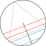
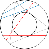
To illustrate: assume that chords are laid at random onto a circle with a diameter of 2, say by throwing straws onto it from far away and converting them to chords by extension/restriction. Now another circle with a smaller diameter (e.g., 1.1) is laid into the larger circle. Then the distribution of the chords on that smaller circle needs to be the same as the restricted distribution of chords on the larger circle (again using extension/restriction of the generating straws). Thus, if the smaller circle is moved around within the larger circle, the restricted distribution should not change. It can be seen very easily that there would be a change for method 3: the chord distribution on the small red circle looks qualitatively different from the distribution on the large circle:

The same occurs for method 1, though it is harder to see in a graphical representation. Method 2 is the only one that is both scale invariant and translation invariant; method 3 is just scale invariant, method 1 is neither.

However, Jaynes did not just use invariances to accept or reject given methods: this would leave the possibility that there is another not yet described method that would meet his common-sense criteria. Jaynes used the integral equations describing the invariances to directly determine the probability distribution. In this problem, the integral equations indeed have a unique solution, and it is precisely what was called "method 2" above, the random radius method.

In a 2015 article, Alon Drory argued that Jaynes' principle can also yield Bertrand's other two solutions. Drory argues that the mathematical implementation of the above invariance properties is not unique, but depends on the underlying procedure of random selection that one uses (as mentioned above, Jaynes used a straw-throwing method to choose random chords). He shows that each of Bertrand's three solutions can be derived using rotational, scaling, and translational invariance, concluding that Jaynes' principle is just as subject to interpretation as the principle of indifference itself.

For example, we may consider throwing a dart at the circle, and drawing the chord having the chosen point as its center. Then the unique distribution which is translation, rotation, and scale invariant is the one called "method 3" above.

Likewise, "method 1" is the unique invariant distribution for a scenario where a spinner is used to select one endpoint of the chord, and then used again to select the orientation of the chord. Here the invariance in question consists of rotational invariance for each of the two spins. It is also the unique scale and rotation invariant distribution for a scenario where a rod is placed vertically over a point on the circle's circumference, and allowed to drop to the horizontal position (conditional on it landing partly inside the circle).

Physical experiments

"Method 2" is the only solution that fulfills the transformation invariants that are present in certain physical systems—such as in statistical mechanics and gas physics—in the specific case of Jaynes's proposed experiment of throwing straws from a distance onto a small circle. Nevertheless, one can design other practical experiments that give answers according to the other methods. For example, in order to arrive at the solution of "method 1", the random endpoints method, one can affix a spinner to the center of the circle, and let the results of two independent spins mark the endpoints of the chord. In order to arrive at the solution of "method 3", one could cover the circle with molasses and mark the first point that a fly lands on as the midpoint of the chord. Several observers have designed experiments in order to obtain the different solutions and verified the results empirically.

Miscellaneous

Let’s clarify.
Let’s assume that we have a probability space $T=(\Omega \mathrm {,} {\phantom {a}}{\mathcal {T}}\mathrm {,} {\phantom {a}}P)$ which describes the Bertrand’s experiment, where $\Omega$, is the sample set of the chords, and $A\in {\mathcal {T}}$ the event: “To pick up randomly a chord of length greater than p from a unit disk”, $p={\sqrt {3}}$

Since basically a chord is a length and an orientation (see example 4), we expect to define a chord with two parameters, so that we may have a measurable function, $X$: $\Omega {\overset {X}{\longrightarrow }}\Omega _{X}$ with $\Omega _{X}$ subset of $\mathrm {\mathbb {R} } ^{2}$. So the random variable $X$, will have the law $P_{X}{\underset {\mathrm {def.} }{=}}P\mathrm {o} X^{-1}$ on a $\sigma$-algebra ${\mathcal {T}}_{X}$. Then somewhere we hope to find a random variable $\varphi$ mapping the length of the chord, $\varphi$: $\Omega _{X}{\overset {\varphi }{\longrightarrow }}[0$, $2]$. The probability we look for is:

$P(A)=\int _{A}dP=\int _{X(A)}dP_{X}$ with $X(A)=\varphi ^{-1}([p\mathrm {,} 2])$. So in that context no matter what our choice is for $X$, the result $P(A)$, independent of $X$ would be the same (Unless $T$ actually doesn’t exist).

However if we suppose $P_{X}$ to have a constant density such as in examples 1. to 5., that is of density equal to ${\frac {1}{\mu (\Omega _{X})}}1_{\Omega _{X}}$, (If $x\in \Omega _{X}$ then $1_{\Omega _{X}}(x)=1$ and $=0$ otherwise) $\mu$ typically the Borel-Lebesgue measure, which may in turn, allow us to calculate the second member of the equality above such as $\mu {\big (}X(A){\big )}{\big /}\mu (\Omega _{X})$, we might get in trouble (Not to mention that ${\frac {1}{\mu (\Omega _{X})}}$ might be null, see example 6. above) . Because we have no guarantee, nor a shred of evidence this actually be the case. Below is a closer look at what is at stake.

Example 2 or 1 vs example 3

Let’s assume we have the following commutative diagram: function commutative diagram Where, for $j=1$ or $j=2$, $(\Omega \mathrm {,} {\phantom {a}}{\mathcal {T}}\mathrm {,} {\phantom {a}}P)$ a probability space, $\Omega _{j}\subset \mathbb {R} ^{n}\mathrm {,} {\phantom {a}}n$ integer, $K\subset \mathbb {R}$ $(\Omega _{j}\mathrm {,} {\phantom {a}}{\mathcal {T}}_{j}\mathrm {,} {\phantom {a}}P_{X_{j}})$ a probability space, ${\mathcal {T}}_{j}{\underset {\mathrm {def.} }{=}}{\mathcal {T}}_{\mathrm {o} }\cap \Omega _{j}\mathrm {,} {\phantom {a}}{\mathcal {T}}_{\mathrm {o} }$ the Borel $\sigma$-algebra $X_{j}$ a random variable $\varphi _{j}$ measurable for the Borel-Lebesgue measure and the Borel $\sigma$-algebra associated with. $\psi$ differentiable, bijective ${\displaystyle }$ on the interior of $\Omega _{2}$, whose Jacobian ($=\mathrm {det} {\big (}\mathrm {D} (\psi ){\big )}$, $\mathrm {D} (\psi )$ differential) is of constant sign. Assuming that $P_{X_{j}}{\underset {\mathrm {def.} }{=}}P\mathrm {o} X_{j}^{-1}$ has a density $f_{j}$, then for any $B=X_{j}^{-1}(A_{j})\in {\mathcal {T}}$, for $A_{j}$ measurable: $P(B)=\int _{B}dP=\int _{X_{1}(B)}f_{1}=\int _{X_{2}(B)}f_{2}$ In particular: for $K=[0\mathrm {,} {\phantom {a}}2]$ $P(A)=\int _{\varphi _{1}^{-1}{\big (}{\big [}{\sqrt {(}}3)\mathrm {,} {\phantom {a}}2{\big ]}{\big )}}f_{1}=\int _{\varphi _{2}^{-1}{\big (}{\big [}{\sqrt {(}}3)\mathrm {,} {\phantom {a}}2{\big ]}{\big )}}f_{2}$ and: $\int _{X_{1}(B)}f_{1}=\int _{\psi \mathrm {o} X_{2}(B)}f_{1}=\int _{X_{2}(B)}{\Big |}\mathrm {det} (\mathrm {D} (\psi ){\big )}{\Big |}f_{1}\mathrm {o} \psi$ if $\Omega _{2}\setminus \mathrm {interior} (\Omega _{2})$ of null measure. Where $\mathrm {D} (\psi )$ is the differential of $\psi$, so: ${\Big |}\mathrm {det} {\big (}\mathrm {D} (\psi ){\big )}{\Big |}f_{1}\mathrm {o} \psi =f_{2}$${\phantom {blbla}}\mu$-almost everywhere, if $\Omega _{2}\setminus \mathrm {interior} (\Omega _{2})$ of null measure. Application example 2 vs example 3 Example 3: $\Omega _{1}={\mathcal {D}}_{1}$, density law equal to $f_{1}$, $\varphi _{1}:{\begin{cases}{\mathcal {D}}_{1}&\to [0\mathrm {,} 2]\\(x\mathrm {,} {\phantom {a}}y)&\mapsto 2(1-x^{2}-y^{2})^{\frac {1}{2}}\end{cases}}$ Example 2: $\Omega _{2}=[0\mathrm {,} {\phantom {a}}1]\mathrm {x} [0\mathrm {,} {\phantom {a}}1[$, density law equal to $f_{2}$, $\varphi _{2}:{\begin{cases}{[}0\mathrm {,} {\phantom {a}}1]\mathrm {x} [0\mathrm {,} {\phantom {a}}1[&\to [0\mathrm {,} 2]\\(r\mathrm {,} {\phantom {a}}\theta )&\mapsto 2(1-r^{2})^{\frac {1}{2}}\end{cases}}$ $K=[0\mathrm {,} {\phantom {a}}2]$, $\varphi _{j}$ gives the length of the chord. $\psi :{\begin{cases}{]}0\mathrm {,} {\phantom {a}}1]\mathrm {x} [0\mathrm {,} {\phantom {a}}1[&\to {\mathcal {D}}_{1}\setminus \{\mathrm {O} \}\\(r\mathrm {,} {\phantom {a}}\theta )&\mapsto (r\cos(2\pi \theta )\mathrm {,} {\phantom {a}}r\sin(2\pi \theta ))\end{cases}}$ $\mathrm {D} (\psi )_{{\big |}(r\mathrm {,} {\phantom {a}}\theta )}={\begin{pmatrix}\cos(2\pi \theta )&-2\pi r\sin(2\pi \theta )\\\sin(2\pi \theta )&2\pi r\cos(2\pi \theta )\end{pmatrix}}$, ${\Big |}\mathrm {det} {\big (}\mathrm {D} (\psi ){\big )}{\Big |}=2\pi r$ Thus $f_{2}=2\pi rf_{1}\mathrm {o} \psi {\phantom {blbla}}\mu$-almost everywhere Now if we choose $f_{1}$ to be constant on ${\mathcal {D}}_{1}$ that is $f_{1}={\frac {1}{\pi }}1_{{\mathcal {D}}_{1}}$ then $f_{2}=2\pi r{\frac {1}{\pi }}1_{\psi ^{-1}({\mathcal {D}}_{1})}=2r1_{[0\mathrm {,} {\phantom {a}}1]^{2}}$ ${\phantom {blbla}}\mu$-almost everywhere, which might challenge the say that "Obviously, in example 2., the density of $P_{X_{2}}$ is a unit constant i.e $f_{2}=1_{[0\mathrm {,} {\phantom {a}}1]^{2}}$, thanks to equiprobability". Especially, if we have already used the same rationale to say that the density $f_{1}$ for $P_{X_{1}}$ is constant thanks to equiprobability. P.S. : ${\phantom {{\bigg (}=}}\int _{[0\mathrm {,} {\phantom {a}}{\frac {1}{2}}]\mathrm {x} [0\mathrm {,} {\phantom {a}}1[}2rdrd\theta ={\frac {1}{4}}$ ${\bigg (}=\int _{\varphi _{1}^{-1}([{\sqrt {3}}\mathrm {,} {\phantom {a}}2])}f_{1}=\int _{{\mathcal {D}}_{\frac {1}{2}}}{\frac {1}{\pi }}dxdy{\bigg )}$ Application example 1 vs example 2 Example 1: $\Omega _{2}={\big [}0\mathrm {,} {\phantom {a}}{\frac {\pi }{2}}{\big ]}\mathrm {x} {\big [}0\mathrm {,} {\phantom {a}}1{\big [}$, density law equal to $f_{2}$, $\varphi _{2}:{\begin{cases}{\big [}0\mathrm {,} {\phantom {a}}{\frac {\pi }{2}}{\big ]}\mathrm {x} [0\mathrm {,} {\phantom {a}}1{\big [}&\to {\big [}0\mathrm {,} {\phantom {a}}2{\big ]}\\(\alpha \mathrm {,} {\phantom {a}}\nu )&\mapsto 2\cos(\alpha )\end{cases}}$ Example 2: $\Omega _{1}={\big [}0\mathrm {,} {\phantom {a}}1{\big ]}\mathrm {x} {\big [}0\mathrm {,} {\phantom {a}}1{\big [}$, density law equal to $f_{1}$, $\varphi _{1}:{\begin{cases}{\big [}0\mathrm {,} {\phantom {a}}1{\big ]}\mathrm {x} {\big [}0\mathrm {,} {\phantom {a}}1{\big [}&\to {\big [}0\mathrm {,} {\phantom {a}}2{\big ]}\\(r\mathrm {,} {\phantom {a}}\theta )&\mapsto 2(1-r^{2})^{\frac {1}{2}}\end{cases}}$ $K={\big [}0\mathrm {,} {\phantom {a}}2{\big ]}$, $\varphi _{j}$ gives the length of the chord. $\psi :{\begin{cases}{\big ]}0\mathrm {,} {\phantom {a}}{\frac {\pi }{2}}{\big ]}\mathrm {x} {\big [}0\mathrm {,} {\phantom {a}}1{\big [}&\to {\big [}0\mathrm {,} {\phantom {a}}1{\big ]}\mathrm {x} {\big [}0\mathrm {,} {\phantom {a}}1{\big [}\\(\alpha \mathrm {,} {\phantom {a}}\nu )&\mapsto {\big (}\sin(\alpha )\mathrm {,} {\phantom {a}}\nu +{\frac {\alpha }{2\pi }}-{\frac {1}{4}}{\big )}\end{cases}}$ $\psi$ calculation details. ${\phantom {aaaaaaa}}$The $\psi$ function For $r(\alpha$, $\nu )$: Thales. For $\theta (\alpha$, $\nu )$:$M$ on the circle and $D_{\alpha }$, $O$ center of the circle, ${\vec {u}}=\exp(2\pi i\theta )$, $\omega =O+r{\vec {u}}$, ${\overset {\longrightarrow }{\omega M}}.{\vec {u}}=0$. $({\overset {\longrightarrow }{\omega O}}+{\overset {\longrightarrow }{OM}}).{\vec {u}}=0$, ${\overset {\longrightarrow }{O\omega }}.{\vec {u}}=r\rightsquigarrow {\overset {\longrightarrow }{OM}}.{\vec {u}}=r$, ${\overset {\longrightarrow }{OM}}=\exp(2\pi i\nu )$, $\cos {\big (}2\pi (\theta -\nu ){\big )}=r=\sin \alpha \rightsquigarrow$ $\theta (\alpha \mathrm {,} {\phantom {a}}\nu )=\nu +{\frac {\alpha }{2\pi }}-{\frac {1}{4}}$. $\mathrm {D} (\psi )_{{\big |}(\alpha \mathrm {,} {\phantom {a}}\nu )}={\begin{pmatrix}\cos(\alpha )&0\\{\frac {1}{2\pi }}&1\end{pmatrix}}$, ${\Big |}\mathrm {det} {\big (}\mathrm {D} (\psi ){\big )}{\Big |}=\cos(\alpha )$ $f_{2}=\cos(\alpha )f_{1}\mathrm {o} \psi$, ${\phantom {a}}\mu$-almost everywhere. Now if we say that the density $f_{1}$ is constant thus equal to $1_{{\big [}0\mathrm {,} {\phantom {a}}1{\big ]}\mathrm {x} {\big [}0\mathrm {,} {\phantom {a}}1{\big [}}$, such as in example 2 then it renders for example 1. of density $f_{2}$, without a shadow of a doubt: $\int _{{\big [}0\mathrm {,} {\phantom {a}}{\frac {\pi }{6}}{\big ]}\mathrm {x} {\big [}0\mathrm {,} {\phantom {a}}1{\big [}}f_{2}=\int _{{\big ]}0\mathrm {,} {\phantom {a}}{\frac {\pi }{6}}{\big ]}\mathrm {x} {\big [}0\mathrm {,} {\phantom {a}}1{\big [}}\cos(\alpha )f_{1}\mathrm {o} \psi =\int _{{\big ]}0\mathrm {,} {\phantom {a}}{\frac {\pi }{6}}{\big ]}\mathrm {x} {\big [}0\mathrm {,} {\phantom {a}}1{\big [}}\cos(\alpha )d\alpha d\nu ={\frac {1}{2}}$

One way out is to define a chord as a choice of two points on a circle, because assuming for each of them that they follow a unit density probability is not so far-fetched and since this latter depends on the structure of the circle only, and not how we sketch up a chord whatsoever, this should do the job.

A way out

The unit circle $S_{1}={\big \{}u\in \mathrm {\mathbb {R} } ^{2}/\|u\|=1$, $\|.\|$ the Euclidean norm ${\big \}}$ is homeomorphic to $\mathrm {\mathbb {R} /\mathbb {Z} }$. On $\mathrm {\mathbb {R} /\mathbb {Z} }$ we use the measure $\delta$ of density 1, which corresponds to the length divided by $2\pi$ of an arc modulo 1, on $\mathrm {\mathbb {R} /\mathbb {Z} }$. More formally: We have the following commutative diagram. Commutative diagram for exp(2πiθ) function With $\phi (\theta )=\mathrm {exp} (2\pi i\theta )$ ${\big (}\mathbb {C} \thicksim \mathbb {R} ^{2}\mathrm {,} {\phantom {a}}i^{2}=-1{\big )}$, $\varphi$ homeomorphism, $\Pi$ the canonical projection. We define an arc, as the image of a continuous injective function, $\gamma :[0\mathrm {,} {\phantom {a}}1]\longrightarrow \mathrm {\mathbb {R} /\mathbb {Z} }$ . $p$ the restriction of $\Pi$ on $[0\mathrm {,} {\phantom {a}}1[$, $p=\Pi _{|[0\mathrm {,} 1[}$ is bijective: $p$ is surjective: $p([0$, $1[)=\varphi ^{-1}\mathrm {o} \phi ([0$, $1[)=\varphi ^{-1}(S_{1})=\mathbb {R} /\mathbb {Z}$. $p$ is injective: $x$, $y\in [0$, $1[$ such that $p(x)=p(y)$, $\Pi (x)=\Pi (y)$, $x-y\in \mathbb {Z}$, $x=y$ And we denote ${\mathcal {T}}_{\mathrm {arc} }$ the $\sigma$-algebra generated by the arcs of $\mathrm {\mathbb {R} /\mathbb {Z} }$. $\Pi$ is continuous ${\big (}F$ a closed set of $\mathrm {\mathbb {R} /\mathbb {Z} }$, $\Pi ^{-1}(F)=\phi ^{-1}\mathrm {o} \varphi (F)\mathrm {,} {\phantom {a}}F$ closed in compact, compact, $\varphi (F)$ compact hence closed, eventually, $\phi ^{-1}{\big (}\varphi (F){\big )}$closed${\big )}$, and so the restriction of $\Pi$ to $]0\mathrm {,} {\phantom {a}}1[$ also and${\phantom {a}}p$ is but maybe in $0$. Then $\delta =\mu \mathrm {o} p^{-1}$ is a measure on $(\mathrm {\mathbb {R} /\mathbb {Z} } }\mathrm {,} {\phantom {a}}{\mathcal {T_{\mathrm {arc} })}$. And since $\delta (\mathbb {R} /\mathbb {Z} )=\mu \mathrm {o} p^{-1}(\mathbb {R} /\mathbb {Z} )=\mu ([0\mathrm {,} {\phantom {a}}1[)=1$, $(\mathrm {\mathbb {R} /\mathbb {Z} } \mathrm {,} {\phantom {a}}{\mathcal {T}}_{\mathrm {arc} }\mathrm {,} {\phantom {a}}\delta )$ is a probability space. And our best bet is to choose it as the probability space of the experiment consisting of randomly picking a point on a circle. With that the probability a point lies on a sector of size $2\pi \Delta$ radian would be $\Delta \in [0$, $1]$. Typically $\mathrm {Im} (\gamma )$ an arc, if $p^{-1}{\big (}\mathrm {Im} (\gamma ){\big )}=[\theta _{1}$, $\theta _{2}]$ then $\delta {\big (}\mathrm {Im} (\gamma ){\big )}=\delta \mathrm {o} p([\theta _{1}\mathrm {,} \theta _{2}])=\mu ([\theta _{1}\mathrm {,} \theta _{2}])=\theta _{2}-\theta _{1}$ . Now let's consider: $p^{-1}:\mathbb {R} /\mathbb {Z} \longrightarrow$ $[0$, $1[$. $p^{-1}$ is bijective, and continuous on $p(]0$, $1[)$. $p^{-1}$ is continuous on $p(]0$, $1[)$: Let $K$ be a compact in $p(]0$, $1[)$. $p^{-1}(K)$ closed, bounded thus compact. for $F$ a closed set $\subset p^{-1}(K)$, $F$ compact, $\varphi ^{-1}\mathrm {o} \phi (F)=p(F)$ compact, thus closed. Hence, $p^{-1}$ is continuous on any compact of $p(]0$, $1[)$. Let be $x\in p(]0$, $1[)$, $p^{-1}(x)\in ]0$, $1[$, there exists a compact $K$ such that $p^{-1}(x)\in K\subset ]0$, $1[$, $x\in p(K)$ compact, $p^{-1}$ continuous in $x$. Henceforth, $\delta \mathrm {o} p$ is a measure on the measurable space $([0$, $1[$, ${\mathcal {T}}_{1})\mathrm {,} {\phantom {aa}}{\mathcal {T}}_{1}={\mathcal {T}}_{\mathrm {o} }\cap [0$, $1[$, ${\mathcal {T}}_{\mathrm {o} }$ the Borel $\sigma$-algebra. . $\delta \mathrm {o} p=\mu _{|_{[0\mathrm {,} {\phantom {a}}1[}}$, that is, $A$ a borel of $\mathbb {R}$: $\mu _{|_{[0\mathrm {,} {\phantom {a}}1[}}(A)=\mu {\big (}A\cap [0\mathrm {,} {\phantom {a}}1[{\big )}=\int _{A}1_{[0\mathrm {,} {\phantom {a}}1[}d\mu$, what we generally write for $A\subset [0\mathrm {,} {\phantom {a}}1[$: $\int _{A}d\mu$, $\int _{A}d\mu (x)$ or simpler $\int _{A}dx$. Thus $\delta \mathrm {o} p$ is of unit density $1_{[0\mathrm {,} {\phantom {a}}1[}$, and the probability space: ${\big (}[0$, $1[$, ${\mathcal {T}}_{1}$, $\mu _{|_{[0\mathrm {,} {\phantom {a}}1[}}{\big )}$, describes also the odds of the experiment consisting of picking randomly a point on a circle. And is equivalent to the previous one (If we have an arc $\mathrm {Im} (\gamma )$ then $p^{-1}(\mathrm {Im} (\gamma ))$ will have the same measure in the latter probability space). Let’s go back to our Bertrand’s conundrum. So we posit a chord to be a choice of two points onto the circle $S_{1}$, so basically a chord is an element of $(\mathrm {R/Z} )^{2}$, assuming that the random variable for the two points are independent, we choose the probability space describing the Bertrand's experiment to be the product space: ${\big (}[0$, $1[^{2}$, ${\mathcal {T}}_{1}^{2}$, $\mu _{|_{[0\mathrm {,} {\phantom {a}}1[^{2}}}{\big )}$. What we look for is the value of: $Q=\int _{\varphi {-1}([{\sqrt {3}}\mathrm {,} 2])}d\mu$ where $\varphi$ is the random variable: $\varphi :{\begin{cases}[0\mathrm {,} {\phantom {a}}1[^{2}&\to [0\mathrm {,} {\phantom {a}}2[\\(\theta \mathrm {,} {\phantom {a}}\nu )&\mapsto {\big \|}u-v\|=2{\big |}\sin {\big (}\pi (\theta -\nu ){\big )}{\big |}\end{cases}}$ Where: $u=\mathrm {exp} (2\pi i\theta )\mathrm {,} {\phantom {a}}v=\mathrm {exp} (2\pi i\nu )$, with $i^{2}=-1$, $\mathbb {R} ^{2}\thicksim \mathbb {C}$ A chord defined as two angles The Bertrand's event we are looking for is ${\big |}\theta -\nu {\big |}\in B={\big [}\alpha \mathrm {,} {\phantom {a}}1-\alpha {\big ]}$ with $\alpha ={\frac {1}{\pi }}\sin ^{-1}{\Big (}{\frac {\sqrt {3}}{2}}{\Big )}={\frac {1}{3}}$. The random variable $\theta -\nu$ has for law: $\mu _{|_{[0\mathrm {,} {\phantom {a}}1[}}\mathrm {*} \mu _{|_{]-1\mathrm {,} {\phantom {a}}0]}}$, where $*$ is the convolution product. Now, $P_{\theta -\nu }=P_{\nu -\theta }{\phantom {a}}$, since $\mu _{|_{[0\mathrm {,} {\phantom {a}}1[}}\mathrm {*} \mu _{|_{]-1\mathrm {,} {\phantom {a}}0]}}=\mu _{|_{]-1\mathrm {,} {\phantom {a}}0]}}\mathrm {*} \mu _{|_{[0\mathrm {,} {\phantom {a}}1]}}$ $(P$ designates $\mu _{|_{[0\mathrm {,} {\phantom {a}}1[^{2}}}$, here$)$, just rename $\theta$ in $\nu$ and vice versa. The probability we look for is: $Q=2\int _{(\theta -\nu )\in B}d{\big (}\mu _{|_{[0\mathrm {,} {\phantom {a}}1[}}\mathrm {*} \mu _{|_{]-1\mathrm {,} {\phantom {a}}0]}}{\big )}=2\int _{\widetilde {B}}d\mu (\theta )d\mu (\nu )\mathrm {,} {\phantom {a}}(=$two times the measure of the area of ${\widetilde {B}})$, where ${\widetilde {B}}={\big \{}(\theta \mathrm {,} {\phantom {a}}\nu )\in [0\mathrm {,} {\phantom {a}}1[^{2}$ such that $\theta -\nu \in B{\big \}}$. Using Fubini since the measures are finite leads to: $Q=2\int _{0}^{\alpha }{\bigg (}\int _{\nu +\alpha }^{1-\alpha +\nu }d\theta {\bigg )}d\nu +2\int _{\alpha }^{1-\alpha }{\bigg (}\int _{\nu +\alpha }^{1}d\theta {\bigg )}d\nu =2{\Big (}{\frac {1}{2}}-\alpha {\Big )}={\frac {1}{3}}$ ${\phantom {aaaaaaa}}$The ${\widetilde {B}}$ area

Bertrand's precept, which states that probability rarely appears as an obvious or intuitive concept, is truer than ever. If we assume that the laws of probability are self-evident or straightforward and rely too much on intuition, we risk treading on quicksand and are bound to encounter messy outcomes, such as paradoxes.

Further reading

• Clark, Michael (2012), Paradoxes from A to Z (3rd ed.), Routledge, ISBN 978-0-415-53857-2
• Gyenis, Zalán; Rédei, Miklós (1 June 2015), "Defusing Bertrand's Paradox", British Journal for the Philosophy of Science, 66 (2): 349–373, doi:10.1093/bjps/axt036, archived from the original on 5 August 2014

External links

• Weisstein, Eric W. "Bertrand's Problem". MathWorld.
• Bertrand's Paradox and More on Bertrand's Paradox by Numberphile & 3Blue1Brown